Tile2Vec on Landsat 7 Satellite Imagery

Update: May 2018: SustainLab’s Tile2Vec paper accepted to AAAI Conference on Artificial Intelligence (AAAI), 2019.

In the following tutorial, I detail how to use Tile2Vec with Landsat 7 satellite imagery and apply it to predicting consumption expenditures in Uganda. Preliminary work yields an average \(r^2\) slightly better than a previous baseline established in Nature. Results near the end of May 2018 are summarized in our submission here.

Many thanks to Marshall Burke, Neal Jean, and Sherrie Wang for their mentorship. Thanks also to Anthony Perez, David Lobell, and Stefano Ermon for helpful pointers and advice.

A lot of the original code can be found in Neal Jean and Sherrie Wang’s original Tile2Vec repo and Neal Jean’s predicting poverty repo, in which he used transfer learning for the same prediction task. Both Neal and Sherrie are the original developers of Tile2Vec. My fork is a combination of these repos along with some edits and extensions that I wrote.

Overview
Model
Setting Up
Gathering Data
Running Experiments
Helpful Links

Overview

Tile2Vec is based on a simple idea: two images which are geographically close together should have embeddings which are close together. How good are these embeddings and can they be used for a variety of downstream tasks?

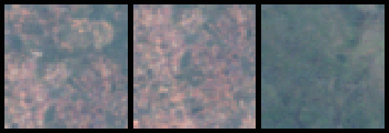
_{Two images which should be close in embeddings and one further away (Google Earth Engine)}

In this tutorial, I explore the capabilities of this model and evaluate it on predicting household level spend in Uganda. Here is a description of the task from the paper:

To measure how well these embeddings predict poverty, we use the World Bank Living Standards Measurement Surveys (LSMS). This survey, conducted in Uganda in 2011-12, samples clusters throughout the country based on population and then randomly surveys households within each cluster. Per capita expenditures within each cluster are averaged across households. The final dataset includes 315 clusters.

To learn embeddings, we use imagery from the Landsat 7 satellite. Landsat 7 is a 1999 satellite that gathers multi-spectral data of the Earth’s surface in 16 day periods. Among other bands, each image includes red, green, blue, near infrared, and short-wave infrared bands at 30 meter spatial resolution. We gather Landsat images from Uganda by bounding Uganda in a rectangular region and taking median composites from 2009-2011 using Google Earth Engine’s Landsat SimpleComposite tool. We then create triplets using two images (tiles) that are geographically close together and an image (tile) that is far away.

Model

Letting \((a,n,d)\) refer to the anchor, neighbor, and distant tiles, we learn embeddings by minimizing the following triplet loss:

where \(m\), the margin, is a hyperparameter of the model. Here, \(f\) is a deep neural network model. \(f(a)\) is the embedding for image \(a\). For this tutorial, \(f\) will often be some variant of a ResNet. You can see different models in our repo’s data/src/ but as of now, most are variants of the ResNet architecture.

Results

For the paper, we trained Tile2Vec on 100k such triplets for 50 epochs using a margin of 50, 0.01 l2 regularization, and Adam optimizer with a 1e-3 learning rate and betas (0.5, 0.999). We used src/tilenet.py as the model. The output embedding has 512 dimensions. Here is a paper excerpt on the results:

The previous state-of-the-art result used a transfer learning approach in which a CNN is trained to predict nighttime lights (a proxy for poverty) from daytime satellite images — the features from this model are then used to predict consumption expenditures [11]. We use the same LSMS pre-processing pipeline and ridge regression evaluation (see [11] for details). Evaluating over 10 trials of 5-fold cross-validation, we report an average \(r^2\) of 0.496 ± 0.014 compared to \(r^2 = 0.41\) for the transfer learning approach — this is achieved with publicly available daytime satellite imagery with much lower resolution than the proprietary images used in [11] (30 m vs. 2.4 m).

Note that following previous work on this dataset, we are predicting log consumption expenditures instead of consumption expenditures.

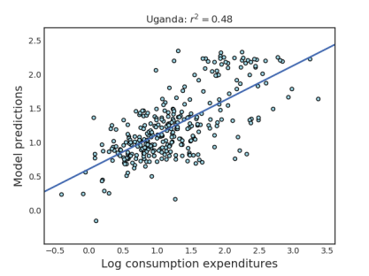
_{Figure A4 from the paper}

For more details on the application, LSMS dataset, and the previous state of the art, please see “Combining Satellite Imagery and Machine Learning to Predict Poverty” by Jean, Burke, et al. and their supplementary material.

Note: Further look ahe original state of the art paper both reports a .41 and .46 r2 and it is unclear what the .41 is trained on. Either way, Tile2Vec is still better than this, and future work that uses nightlights might yield even better results.

Setting Up

The majority of code has been taken from two repositories (see links above) connected to this project and placed into a fork specific for this application.

Grab the repo:

git clone https://github.com/anshulsamar/tile2vec.git

Change the paths to point to your directories by editing paths.py. Here is what I did to setup on a clean instance- this isn’t everything and I need to update the environment file to include more things, but will hopefully get new students started. The following instructions are for Ubuntu 16.04.4 LTS on a Google Cloud Compute instance with 8 vCPUs, 52 GB memory, 1 NVIDIA Tesla P100, and Intel Broadwell CPU platform.

1. sudo apt-get update
2. sudo apt-get install emacs24 Sorry, vim friends.
3. sudo apt-get install gcc
4. Install Cuda.
5. Install Anaconda, tutorial here.
6. conda update -n base conda
7. cd tile2vec
8. conda env create -f environment.yml
9. Activate environment: source activate tile2vec (alias this later)
10. Install PyTorch. For me, the correct command was conda install pytorch torchvision cuda91 -c pytorch
11. conda install -c menpo imageio
12. Install pip: sudo apt-get install python3-pip
13. Use pip to install tensorboardX (I think you will need to also install tensorflow and normal tensorboard for this).
14. Install Torch Summary (to output summaries of model files) pip install torchsummary

For gcloud users, download and initialize gcloud so you can transfer data to and from buckets. It may be helpful for your experiments to use screen that way you can exit from your SSH session and still have the process running. See this link about screen and this link for using screen as a different user.

Gathering Data

In this section, we’ll gather data for all of Uganda - to be used in the Tile2Vec unsupervised task - and also data specific to LSMS locations. If you haven’t already, go ahead and sign up for a Earth Engine developer account here.

Both earth engine scripts referenced below extract Landsat 7 satellite imagery. For every location in Uganda, images are extracted for years 2009-2011 and then composited together using the ee.Algorithms.Landsat.simpleComposite() method. According to the documentation: “This method selects a subset of scenes at each location, converts to TOA reflectance, applies the simple cloud score and takes the median of the least cloudy pixels.”

Uganda Data

Use the data/uganda_earthengine.js script to download tif files of Landsat 7 satellite imagery of Uganda from Google Earth Engine. Make sure to create a bucket on your Google Cloud account that the images can be exported to. With this code viewer, you may have to manually click run on the task bar for every exported image - there is also a python API that may be easier.

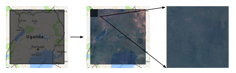
_{Uganda and Landsat 7 satellite imagery (Google Earth Engine)}

In the current script, the downloaded tif files will have large dimensions and will need to be convered to npy. Run python process_data.py to grid each tif file into smaller patches. For the Uganda data, this yields \(2^{14}\) squares of \(145 \times 145 \) pixels each.

To do: currently the channel dimension is moved to the end and then moved back later during training, this can perhaps be simplified. Furthermore, process_data is legacy and was done to deal with large tif images- the data can be exported from Google Earth Engine in smaller dimensions and this step can be avoided

Note: the original tif tiles may not be perfectly divisible by the desired width/height of small patches created by process_data.py. The excess pixels are ignored

After this, divide up these patches into train and test set:

mkdir [paths.train_images]
mkdir [paths.test_images]
mv `ls [home_dir]/data/npy/ | shuf | head -NUM` paths.train_images
mv home_dir/data/npy/*.npy paths.test_images

I kept only 1024 (\(2^{10}\)) patches in test and moved the rest to train to get more area coverage.

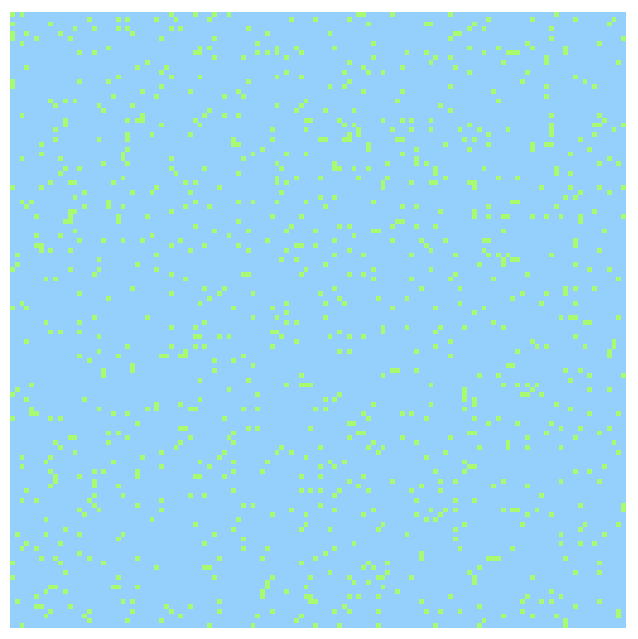
_{Train Test Split (train triplets sampled from blue, test from green)}

Once the data is in your data/npy/train and data/npy/test folder, we are now ready to make triplets. At a high level, each triplet requires an anchor, neighbor, and distant image. Anchor and neighbor images come from the same \(145 \times 145\) patch and are required to be within a certain neighborhood of one another. The distant image comes from another random patch in the set.

The -val command creates a validation set that uses the same underlying npy images as the training set (the blue color above). Note, this is no different than creating more training triplets and then splitting them into a train and val set.

python make_triplets.py -train --ntrain 500000 -test --ntest 100000
-val --nval 100000 

These triplets will be stored in data/tiles folder.

To see some examples of triplets, run python visualize.py. This will post triplets to TensorBoard for viewing. There is also an experimental embeddings visualizer that uses the most recent set of features in paths.lsms_data to create a 3D embedding. This still needs to be worked on, but go to the “projector” tab of TensorBoard to check it out.

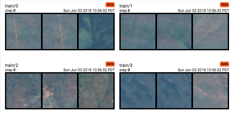
Here are some triplet examples from the training set:

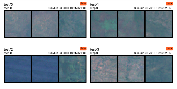
From the test set:

LSMS Data

Use the code in data/lsms_earthengine.js to extract patches around LSMS locations. You can change the box width and height depending on how large you want each patch to me (it will be roughly centered around the coordinate point in the LSMS dataset).

If you like, you can also create a triplet training set purely from images taken from these LSMS locations. You can adjust the box width and box height in the Earth Engine script to change how large you want these LSMS images to be. In my current setup, there are separate folders for large and small LSMS tif images. These images do not require conversion to npy.

Todo: this process and the above process needs to be streamlined so conversions are not required.

python make_triplets.py -lsms_train --nlsms_train 500000 -lsms_val
100000 --nlsms_val 100000

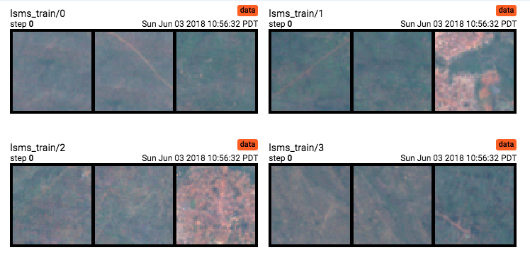
Here are some triplets from the LSMS train set:

Running Experiments

To train, use the run.py file. Example:

python run.py --model minires_32 --z_dim 32 --exp_name minires_32_500K
-train --ntrain 500000 -val -test -predict_small --trials 5 -save_models

This will use the minires_64 model with 34 dimensions. It will train on 250000 triplets and validate and test on the default sets. It will go into test mode to predict LSMS data. To do this, embeddings will be created for LSMS images and then used in a ridge regression model. This will be done for 5 trials and the average \(r^2\) will be outputted. Models and loss will be saved every epoch.

There are multiple prediction modes. -predict_small uses small crops around LSMS locations and samples 10 \(50 \times 50\) tiles in the image. Embeddings from these are averaged and used in ridge regression. -predict_big uses large crops, tiles them into a grid of 36 \(50 \times 50\) tiles. Embeddings from those are averaged and used in regression. Either of these modes can also be used with the -quantile flag which rather than just average embeddings, creates a feature vector with various quantiles.

You can also use the poverty_plot.py file to create a graph of \(r^2\) versus consumption expenditure (similar to Fig A of the original science paper on LSMS data). All other plots are easily seen on your TensorBoard.

Some notes and unfortunate things to look out (these all need to be improved and are minor fixes):

1. Deprecated cross validation scipy warning (you’ll see the warning when running code).

2. Running poverty plot is getting a runtime warning and encountering some invalid values. Started looking into this, but wasn’t able to track it down.

3. fig_utils.py is what runs the regression code and cross validation. I got these functions from the original predicting poverty repo, removing ones and I did not need and making minor edits.

4. Optimization state not being saved

Here are some some results from example experiments. Test and Validation are 50K triplets each.

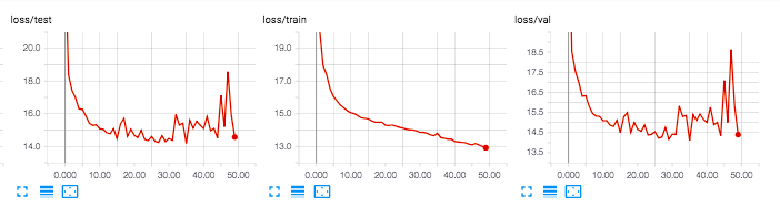
_{A mini version of ResNet that outputs 32 dimensions. Trained on 100K triplets.}

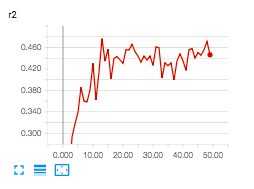
_{r^2 on LSMS data.}

Here are a variety of other experiments testing the model (mini version of resnet vs normal tile2vec architecture), training set size (100K, 250K, 500K), training set images (only LSMS images vs sampling from all over Uganda). These are only some experiments and do not cover all combinations; more need to be done. If you are interested in details, please let me know, happy to share these results/tensorboard log files. These experiments were done on p100 gpu, displayed via Tensorboard, ~0.7 smoothing in display.

Comparing these is a little tricky - ideally the end product would use the best performing model across any epoch (which seems to be tilenet_512_lsms_100K at epoch 7 with .519 r2). This refers to a normal tilenet architecture (resnet), trained only 100K triplets extracted from lsms locations. Similar performance is also found in a mini resnet with only 32 dimensions output trained on 250K triplets sampled from all over Uganda.

_{More Experiments}

For those interested in continuing this work, please feel free to reach out! I have a separate document of unresolved issues (had some strange performances on test) and future experiments to try, happy to discuss those and brainstorm.

Helpful Links

Check out the Tile2Vec paper here and the original work done on LSMS predictions by the lab here (Science Paper) and here (Supplementary material).

[1] Lat/Lon Calculator

[2] Bands in Landsat (USGS)

[3] Landsat 7 Overview.

[4] Landsat 7 Data Users Handbook.

[5] Introduction to Remote Sensing

[6] Understanding Color Infrared Photographs.

[7] Using Google Earth Engine with Landsat

[8] Stereo Matching w/ CNN (Zbontar and LeCun)

[9] World Population Dataset from Google.

[10] Other Datasets from Google.