Inverse Graphics Networks and VAE

In this post, I walk through Kingma and Welling’s Variational Auto-Encoding paper and discuss an application in Deep Inverse Graphics Networks. These are based on my written notes from a tutorial talk to the Stanford Deep Learning on Inverse Graphics Networks.

Introduction
Auto-Encoding Variational Bayes
Reparameterization
Putting it Together
Application: Inverse Graphics Networks

Introduction

Let \(X = {x^{(i)}}_{i=1}^N \) be a dataset. Data points \( x^{(i)} \) are independently and identically distributed samples from the following process:

1. Sample \( z^{(i)} \sim P_\theta(z)\) from the prior.
2. Sample \( x^{(i)} \sim P_\theta(x|z)\) from the likelihood.

Assume that \(P\) is differentiable.

What questions can we ask?

1. Which underlying \(P\) distribution best describes this dataset? (i.e. for gaussian distribution, what are the best \(\mu\) and \(\sigma\)?).
2. What is the posterior distribution \(P_{\theta}(z|x)\)? This is useful for determining the underlying “representation” of a data point.

Say we knew which hidden variable corresponded to which \(x^{(i)}\). Then we could determine \(P_\theta(x,z) = P_\theta(x|z)P_\theta(z)\) for every \(x\). The likelihood of our dataset would be \(\prod_i P_\theta(x^{(i)}|z^{(i)})P_\theta(z^{(i)})\) and the log likelihood, \(\sum_i log(P_\theta(x^{(i)}|z^{(i)})) + log(P_\theta(z^{(i)})) \). We would set this equal to zero, take derivatives, and determine the \(\theta\) that maximize the likelihood under our chosen distribution.

Because we do not know which hidden variable corresponds to which data point, our log likelihood is \(\sum_i log (\int P_\theta(x|z) P_\theta(z) dz)\) and this nasty log of sums becomes difficult to work with (see mixture of gaussian reference below for an example of this).

One might suggest using the EM algorithm and the posterior distribution to iteratively estimate \(\theta\). But what if we wish to use likelihoods and posteriors that are intractable (i.e. no closed form or too computationally expensive)? As Kingma and Welling write, “intractabilities are quite common and appear in cases of moderately complicated likelihood functions \(p_\theta(x|z)\), e.g. a neural network with a nonlinear hidden layer” [1]. For example, in order to determine the marginal likelihood of x, we would need to sweep over all possible values for \(z\), i.e.: \(P_\theta(x) = \int P_\theta(z)P_\theta(x|z)dz \). If the likelihood is given to us by a neural network, this becomes very difficult to determine (as a simple exercise, look at the likelihood given by two sigmoid units connected to each other). The posterior \(P_\theta(z|x) = \frac{P_\theta(x|z)P_\theta(z)}{P_\theta(x)}\) becomes similarly difficult to compute. Even if we were to sample, this would take too long due to the size of our dataset.

How do we find the parameters for our underlying distribution when all we know is our original dataset \(X\)?

Auto-Encoding Variational Bayes

Let’s try to find a function \(q_\phi(z|x)\) that is very close to our posterior \(P_\theta(z|x)\). Because both \(q\) and \(p\) are probability distributions, we use the KL Divergence as cost. Let’s look at just one data point to start. In the remaining section, I use \(x\) instead of \(x^{(i)}\).

\[\begin{align*} D_{KL}(q_\phi(z|x) || p_\theta(z|x)) &= E_{q_\phi(z|x)}[log \frac{q_\phi(z|x)}{p_\theta(z|x)}] \\ &= E_{q_\phi(z|x)}[log q_\phi(z|x)] - E_{q_\phi(z|x)}[log P_\theta(z,x)] + E_{q_\phi(z|x)}[log P_\theta(x)] \\ &=-(E_{q_\phi(z|x)}[logP_\theta(z,x)] - E_{q_\phi(z|x)}[log q_\phi(z|x)])) + log P_\theta(x) \end{align*}\]

Step 1 is the definition of KL divergence on the respective probability distributions. To go to step 2, we distribute the log, using bayes formula to replace the posterior with the joint probability and prior. To go to step 3, we regroup and use the fact that the prior under P is constant with respect to q (thus, removing the expectation).

The first term in line 3 is called the ELBO: evidence based lower bound. It is based purely on things we know - the “evidence” and our approximate distribution.

Thus, more simply:

\[\begin{align*} logP_\theta(x) &= D_{KL}(q_\phi|p_\theta) + ELBO(\phi, \theta;x) \\ ELBO(\phi, \theta; x) &= E_{q_\phi(z|x)}[logP_\theta(z,x)] - E_{q_\phi(z|x)}[log q_\phi(z|x)]) \end{align*}\]

Another way of seeing the relationship between the log likelihood and ELBO is observing ELBO as a lower bound:

Note that:

\[\begin{align*} log P_\theta(x) &= log \int_z P_\theta(x,z) \\ &= log \int_z P_\theta(x,z) \frac{q_\phi(z|x)}{q_\phi(z|x)} \\ &= log E_{q_\phi(z|x)}[ \frac{P_\theta(x,z)}{q_\phi(z|x)}] \\ &\geq E_{q_\phi(z|x)}[log p_\theta(x,z)] - E_{q_\phi(z|x)}[log q_\phi(z|x)] \\ &= ELBO(\theta, \phi; x) \end{align*}\]

This is also called the variational lower bound. We can rewrite the ELBO in another formulation.

\[\begin{align*} ELBO(\theta, \phi; x) &= E_{q_\phi(z|x)}[-log q_\phi(z|x) + log p_\theta(x,z)] \\ &= -E_{q_\phi(z|x)}[log q_\phi(z|x) - log p_\theta(z) - log p_\theta(x|z)] \\ &= -D_{KL}(q_\phi(z|x) || p_\theta(z)) + E_{q_\phi(z|x)}(P_\theta(x|z)) \end{align*}\]

Step 2 is by spliting the joint distribution into individual components.

Note that by maximizing ELBO, we seek parameters \(\theta, \phi\) that lower \(D_{KL}(q_\phi(z|x) || p_\theta(z))\), while increasing \(E_{q_\phi(z|x)}(P_\theta(x|z))\). Why is this interesting? The KL Divergence term ensures that our approximate posterior is close to our prior over \(z\) (say gaussian). Intuitively, the second term uses the approximate posterior to determine distribution of \(z\)s and use these to reconstruct the original \(x\) under the likelihood distribution. By maximizing ELBO we optimize our parameters to maximize reconstruction.

Maximizing ELBO thus becomes a combination of regularization (against a known prior) and autoencoding. Reguralization ensures that we don’t overfit the distribution of the data.

Reparameterization

How might we tackle maximizing ELBO off the bat? Let’s determine gradients with respect to \(\theta\) and \(\phi\).

It’s nice to work with expectations - as it allows us to sample and then evaluate. How might we find gradients, while still maintaining expectations?

As you can see in [8], the gradient w.r.t. \(\theta\) can be done simply. For \(\phi\), we can use the log derivative trick [6] and push the gradient inside. We can then use Monte Carlo to approximate:

\[\begin{align*} \nabla_\phi E_{q_\phi(z|x)}[f(z)] &= E_{q_\phi(z|x)}[f(z)\nabla_\phi log q_\phi(z|x)] \\ &= \frac{1}{L} \sum f(z) \nabla_phi log q_\phi(z|x) \end{align*}\]

The L refers to L samples from \(q_\phi(z|x)\). Kingma and Welling write that doing this “this exhibits very high variance (see e.g. [BJP12] and is impractical for our purposes.” If using gradient descent methods, for example, high variance can lead to convergence difficulties.

Kingma and Welling propose a reparameterization trick (requires some conditions on the posterior - see paper). Here, rather than sample \(z \sim q_\phi\) we set \(z = g_\phi(x, \epsilon)\) where \(\epsilon \sim p(\epsilon)\). For example, say \(q\) is \(N(\mu, \sigma^2)\). Then instead of directly sampling \(z\), we set \(z = g_\phi(x, \epsilon) = \mu + \sigma*\epsilon\) and sample \(\epsilon \sim N(0,1)\) instead.

Now:

\[E_{q_\phi(z|x)}[f(z)] = E_{p(\epsilon)}[f(g_\phi(\epsilon,x))]\]

This can be approximated by \(\frac{1}{L} \sum_l f(g_\phi(\epsilon_l, x))\) where \(\epsilon_l \sim p(\epsilon)\).

Stefano Ermon’s 228 class [8] has a good discussion of this, but note how now the gradient with respect to \(\phi\) can be pushed into the expectation, allowing us to take Monte Carlo estimates.

Reparameterizing this way leads to less variance [8]. See this post for an empirical example and this thread for more discussion. A differentiable f and g, also means we can take derivatives in our gradient descent setup.

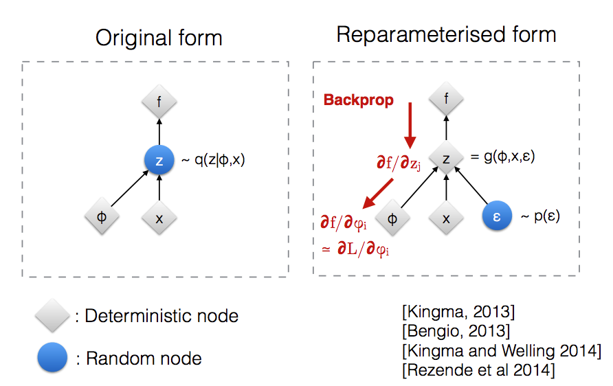
As noted by [7] (original image from Kingma/Welling [9]), this also allows us to backprop.

We can use this trick on either of two ELBO formulations. Doing it on the first formulation leads to the function we want to maximize:

\(ELBO(\theta,\phi;x^{(i)}) \approx \frac{1}{L} \sum_l log P_\theta(x^{(i)},z^l) - log q_\phi(z^l|x^{(i)})\) where \(z^l = g_\phi(\epsilon^l, x^{(i)})\) and \(e^l \sim p(\epsilon)\)

Note that analytic integrations of the KL divergence in the second formulation of ELBO is sometimes possible and can further reduces variance, as we no longer need to use Monte Carlo for that part of the expression.

Putting it Together

We now want to maximize ELBO and use derivatives to update our parameters \(\theta, \phi\). Here is Algorithm 1 from the original paper:

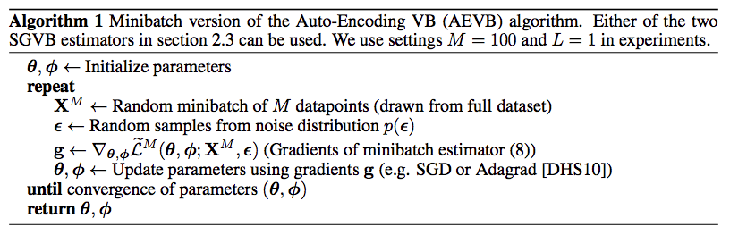
Here \(\tilde L^M\) is \(\frac{N}{M}\sum_i ELBO(\theta,\phi;x^{(i)})\) where \(M\) is the number of points we sample, \(N\) is the size of the dataset, and L is the number of times we sample \(\epsilon\) for each data sample. Here, we use the monte carlo/reparameterized approximation of ELBO from above.

We can take the gradient here as every part of our ELBO, including the reparameterization function, can be differentiated.

Let’s now integrate this into a MLP in the gaussian setting. With a gaussian prior \(p_\theta(z) = N(z;0,I)\) and gaussian posterior, we can get a closed form of the KL divergence term and use the second formulation of ELBO.

Let \(P_\theta(x|z) = N(x; \mu(z), \sigma^2(z)I)\), \(q_\phi(z|x) = N(z, \mu(x), \sigma^2(x)I)\), and \(P_\theta(x|z) = N(x; \mu^{(l)}, \sigma^{2(l)}I)\). Integrating into an autoencoder and using the differentiated closed form, we have (see paper for deriviation details)

Our loss:

\[ELBO(\theta, \phi; x^{(i)} \approx \frac{1}{2} \sum_{j=1}^J (1 + log((\sigma_j^{(i)})^2) - {(\mu_j^{(i)})}^2 - {(\sigma_j^{(i)})}^2) + \frac{1}{L} \sum_l log P_\theta(x^{(i)}|z^{(i,l)}))\]

1. Encoder MLP: \(x \rightarrow \mu(x), \sigma^2(x)\). We can use this to determine the KL divergence part of the loss.
2. \(\mu(x), \sigma^2(x)\) gives us the parameters of the approximate posterior \(q_\phi\). We can then sample \(\epsilon \sim p(\epsilon)\) and set \(z^{(l)} = \mu(x) + \sigma(x)*\epsilon^{(l)}\).
3. Decoder: \(z \rightarrow \mu(z^{(l)}), \sigma^2(z^{(l)})\). This parameterizes our likelihood, \(p_\theta(x|z)\). We can use this to determine the reconstruction part of the loss.

This can be optimized using the AEVB algorithm and backpropagation.

Deep Inverse Convolutional Graphics Networks

In Deep Inverse Convolutional Graphics Networks, we attempt to use an encoder-decoder setup based on variational autoencoding to generate new images of faces. Our goal is to “disentagle” a representation of a face from other independent variables - pose, position, lighting, etc. With traditional autoencoders, we do not have full control over a posterior, but with a generative model, we do. I won’t go into too many details here, but will share some interpretations with those familiar with the work.

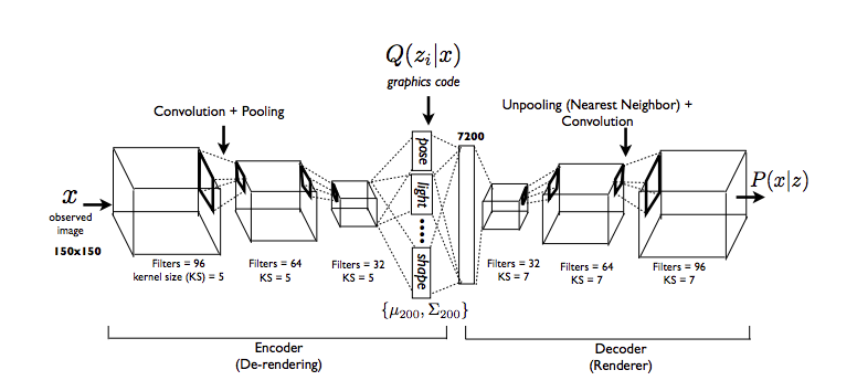
Images from paper [2].

We use a multivariate Gaussian as our approximate posterior. We treat our hidden variable \(z\) as a series of variables - azimuth, face elevation, azimuth of light source, shape, texture, etc. These are called “intrinsic properties.” We proceed in the following steps:

1. Select one such \(z_{train}\) variable at random.
2. Gather a mini-batch only consisting of those images which differ in this variable.
3. Forward propagation. For each example k, sample \(z^{(k)}\). Average them.
4. Replace all variables in z except for the one chosen in step 1 with its mean across examples and push through decoder.
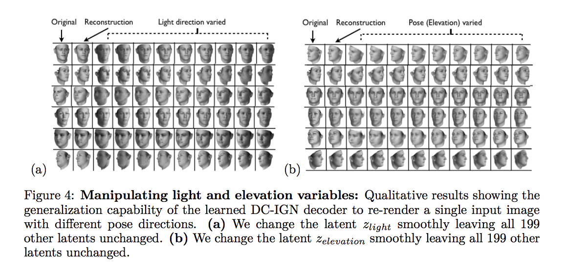
5. Backpropogate decoder/encoder. Here, “Replace the gradients for the latents \(z_i \not= z_{train}\) (the clamped neurons) with their difference from the mean (see Section 3.2). The gradient at ztrain is passed through unchanged.”

What’s awesome is how well this works - we can continuously change latent variables and the samples we draw from the likelihood distribution change to match!

The core intuition is that during training we force other variables to stay the same - as all difference should be explainable by the variable chosen. As an image changes, one neuron (one variable) should be equivariant and change with different data. Others should be invariant.

Can we rationalize this with respect to general autoencoding?

Here is one interpretation: in this setting, rather than learn one autoencoder, we really wish to learn \(n\) autoencoders, one to capture each axes of variation in a paritcular mini-batch. To make this interpretable, we split our dataset into n distinct transformations (each batch corresponds to only one transformation). Then, rather than train \(n\) separate models, we attempt to combine them.

We now need to ensure that the \(z_i\) latent variables inside one batch are the same. We do this by penalizing for variance. For each data point and for each \(z_i \not= z_{train}\), we can add a loss term that penalizes the variance with respect to the others in its mini batch.

\[\begin{align*} L &\mathrel{+}= Var[z_i] \\ &= E[(z_i - E[z_i])]^2 \\ &\approx \frac{1}{L} \sum (z_i - E[z_i])^2 \end{align*}\]

Note that the negative gradient is in the direction of the mean. This is the same as step 5 above.

References

Because the talk happened some time ago and I am writing the post now based on written notes, I don’t remember the references I used outside of the two main papers below. I had taken some bits and insights freely from wikipedia, blogs, and peers, as this was presented in an informal setting, so some language may overlap. Thanks to Ziang Xie, Jonathan Ho, and Kenneth Jung for helpful conversations.

Written based on the following:

[1] Diederik Kingma and Max Welling. Auto-Encoding Variational Bayes. The 2nd International Conference on Learning Representations (ICLR). 2013.

[2] Tejas Kulkarni, William Whitney, Pushmet Kohli, and Joshua Tenenbaum. Deep Convolutional Inverse Graphics Network. NIPS. 2015.

[3] Agustinus Kristiadi. “MLE vs MAP.” wiseodd.github.io. 2017.

[4] Andrew Ng. “The EM Algorithm.” cs229.

[5] Andrew Ng. “Mixtures of Gaussians.” cs229.

[6] Shakir Mohamed. “Log Derivative Trick.” The Spectator.

[7] Reparameterization Trick on Stack Overflow. 2016.

[8] Stefano Ermon Group. VAE.

[9] Diederik Kingma and Max Welling. “Variational Auto-Encoders and Extensions.” NIPS Workshop Talk. 2015.